Introduction: Entropy Is Not Just a Formula
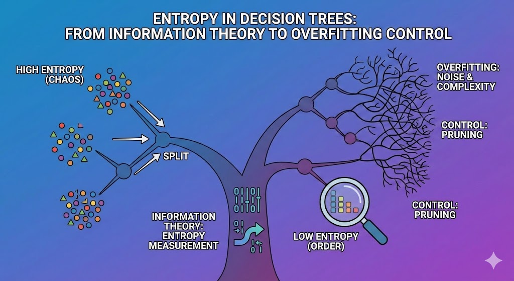
Entropy is often introduced in machine learning as a simple mathematical formula, yet its impact on model behavior is profound. In decision trees, entropy is not merely a metric — it is the driving force behind every split, every branch, and every final prediction.
Understanding entropy deeply explains why decision trees can be both remarkably powerful and dangerously prone to overfitting. This article explores entropy from first principles, connects it to information theory, and shows how uncontrolled entropy reduction leads to memorization rather than learning.
Entropy from an Information Theory Perspective
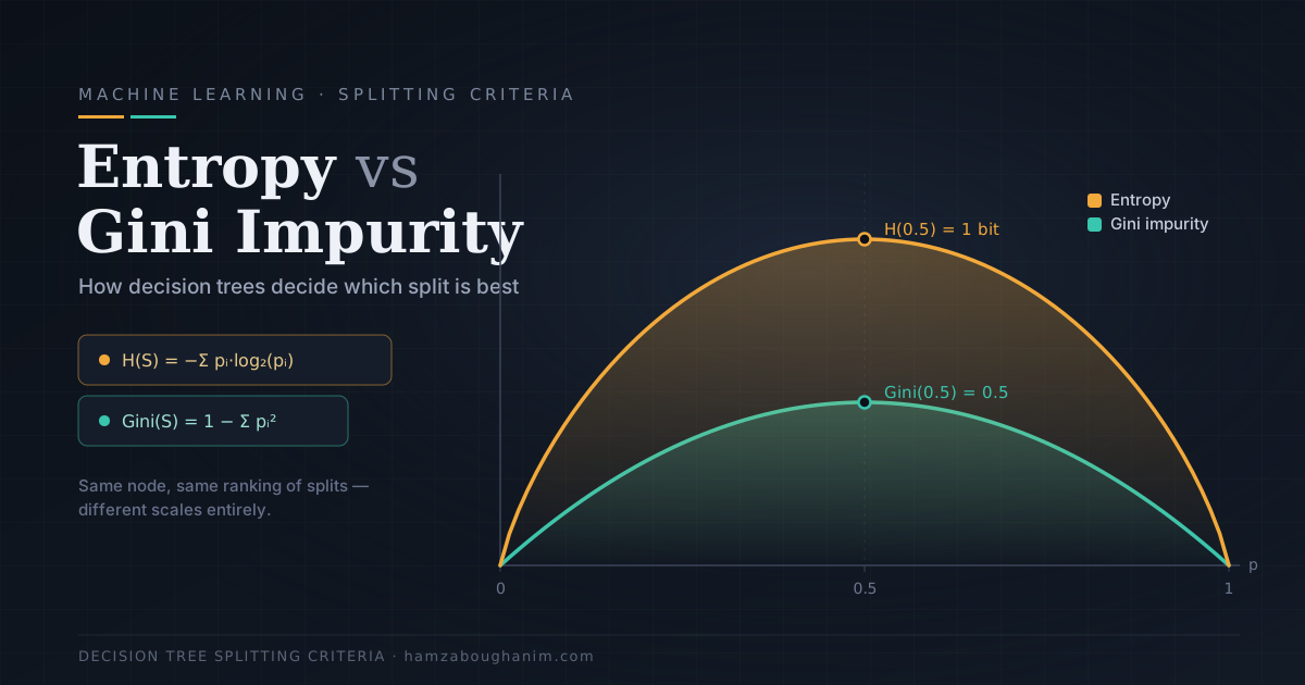
Entropy originates from Shannon's information theory, where it measures the expected amount of information required to describe an outcome. In a classification dataset:
- Low entropy — outcomes are predictable (one class dominates)
- High entropy — outcomes are uncertain (classes are balanced)
Shannon's Entropy Formula
For a node containing samples from C classes with proportions p₁, p₂, … pC:
Entropy(S) = -Σ pᵢ · log₂(pᵢ)

Example — balanced binary split (p = 0.5, 0.5):
  H = -(0.5 · log₂(0.5) + 0.5 · log₂(0.5)) = 1.0 bit   ← maximum uncertainty

Example — pure node (p = 1.0, 0.0):
  H = -(1.0 · log₂(1.0)) = 0.0 bits                      ← perfect certainty
Computing Entropy in Python
import numpy as np

def entropy(y):
    """Shannon entropy of a label array."""
    classes, counts = np.unique(y, return_counts=True)
    probs = counts / counts.sum()
    # Avoid log(0) by masking zero-probability classes
    return -np.sum(probs * np.log2(probs + 1e-12))

# Example
y_balanced  = np.array([0, 0, 0, 1, 1, 1])   # 50/50 split
y_dominated = np.array([0, 0, 0, 0, 0, 1])   # 83/17 split
y_pure      = np.array([1, 1, 1, 1, 1, 1])   # 100% class 1

print(f"Balanced:  {entropy(y_balanced):.4f} bits")    # → 1.0000
print(f"Dominated: {entropy(y_dominated):.4f} bits")   # → 0.6500
print(f"Pure:      {entropy(y_pure):.4f} bits")        # → 0.0000
Why Decision Trees Are Obsessed with Entropy
Decision trees operate under a greedy optimization strategy. At every node, the algorithm asks: which split reduces uncertainty the most? This reduction is quantified using Information Gain.
Information Gain Formula
IG(S, feature) = Entropy(parent) - Σ ( |Sᵥ| / |S| · Entropy(Sᵥ) )

Where Sᵥ are the child subsets created by each value of the feature.
Implementing Information Gain from Scratch
def information_gain(y_parent, splits):
    """
    y_parent : labels in the parent node
    splits   : list of label arrays for each child node
    """
    parent_entropy = entropy(y_parent)
    n = len(y_parent)

    weighted_child_entropy = sum(
        (len(child) / n) * entropy(child)
        for child in splits
    )
    return parent_entropy - weighted_child_entropy

# Example: splitting on a binary feature
y       = np.array([0, 0, 1, 1, 1, 0, 1, 0])
left    = np.array([0, 0, 1])   # feature = 0
right   = np.array([1, 1, 0, 1, 0])  # feature = 1

ig = information_gain(y, [left, right])
print(f"Information Gain: {ig:.4f}")  # → 0.0487
The split that maximizes information gain is selected, pushing the model toward purer and purer subsets — until every leaf contains a single class, or a stopping criterion fires.
The Path to Overfitting
A fully-grown decision tree will reduce entropy to zero on the training set by memorizing every sample individually. This looks like perfect accuracy — but it is the opposite of learning.
The Perfect Purity Trap
As a tree grows deeper, the nature of its splits changes:
- Shallow splits — remove genuine uncertainty from the data
- Deep splits — remove noise, outliers, and random coincidences
When a leaf contains a single sample, its entropy is zero — but the model has learned nothing transferable. It has memorized a data point.
Overfitting Is Entropy Optimization Without Limits
from sklearn.tree import DecisionTreeClassifier
from sklearn.datasets import make_classification
from sklearn.model_selection import train_test_split

X, y = make_classification(n_samples=500, n_features=20, random_state=42)
X_train, X_test, y_train, y_test = train_test_split(X, y, test_size=0.2, random_state=42)

# Unconstrained tree — overfits
tree_full = DecisionTreeClassifier()
tree_full.fit(X_train, y_train)

print(f"Train accuracy: {tree_full.score(X_train, y_train):.3f}")  # → 1.000 (memorized)
print(f"Test  accuracy: {tree_full.score(X_test,  y_test):.3f}")   # → 0.750 (generalized poorly)
print(f"Tree depth:     {tree_full.get_depth()}")                  # → 20+ levels
The model achieves 100% training accuracy because it has reduced entropy to zero for every training sample. But on unseen data, it fails — a classic sign of overfitting.
Controlling Entropy with Structural Constraints
The solution is not to stop entropy reduction entirely, but to constrain when and how far it goes. Scikit-learn exposes several hyperparameters that act as entropy governors.
max_depth — Limiting Information Fragmentation
Each additional depth level multiplies the number of partitions exponentially, fragmenting the dataset into increasingly specific (and statistically unreliable) regions. Limiting depth forces the model to prioritize high-impact splits.
from sklearn.model_selection import cross_val_score

results = []
for depth in [2, 4, 6, 8, 10, None]:
    clf = DecisionTreeClassifier(max_depth=depth, random_state=42)
    cv_score = cross_val_score(clf, X_train, y_train, cv=5).mean()
    results.append((depth, cv_score))
    print(f"max_depth={str(depth):4s} → CV accuracy: {cv_score:.3f}")

# depth=None (unlimited) typically shows the largest gap between train and CV
min_samples_leaf — Statistical Reliability
Entropy does not account for sample size. A leaf with one sample can have zero entropy, yet its prediction is statistically meaningless. Enforcing a minimum ensures that entropy reduction corresponds to reliable evidence, not random chance.
tree_constrained = DecisionTreeClassifier(
    max_depth=6,
    min_samples_leaf=5,   # at least 5 samples per leaf
    random_state=42
)
tree_constrained.fit(X_train, y_train)

print(f"Train accuracy: {tree_constrained.score(X_train, y_train):.3f}")  # → ~0.88
print(f"Test  accuracy: {tree_constrained.score(X_test,  y_test):.3f}")   # → ~0.84
print(f"Tree depth:     {tree_constrained.get_depth()}")                  # → 6
min_impurity_decrease — Rejecting Noisy Splits
Some splits reduce entropy by a negligible amount while dramatically increasing model
complexity. min_impurity_decrease acts as a filter — a split only happens
if the weighted information gain meets the threshold.
tree_impurity = DecisionTreeClassifier(
    min_impurity_decrease=0.01,  # only split if IG >= 0.01
    random_state=42
)
tree_impurity.fit(X_train, y_train)
print(f"Depth: {tree_impurity.get_depth()}, Leaves: {tree_impurity.get_n_leaves()}")
Pruning — Learning When to Forget
Post-pruning takes a fully-grown tree and removes branches that hurt generalization,
even if they improve training accuracy. Scikit-learn implements
cost-complexity pruning via the ccp_alpha parameter.
from sklearn.tree import DecisionTreeClassifier

# Find the optimal alpha using cross-validation
path = DecisionTreeClassifier(random_state=42).cost_complexity_pruning_path(X_train, y_train)
alphas = path.ccp_alphas

best_alpha, best_score = 0, 0
for alpha in alphas:
    clf = DecisionTreeClassifier(ccp_alpha=alpha, random_state=42)
    score = cross_val_score(clf, X_train, y_train, cv=5).mean()
    if score > best_score:
        best_score, best_alpha = score, alpha

print(f"Best alpha: {best_alpha:.5f}, CV score: {best_score:.3f}")

# Train final pruned tree
tree_pruned = DecisionTreeClassifier(ccp_alpha=best_alpha, random_state=42)
tree_pruned.fit(X_train, y_train)
print(f"Pruned depth:  {tree_pruned.get_depth()}")
print(f"Pruned leaves: {tree_pruned.get_n_leaves()}")
print(f"Test accuracy: {tree_pruned.score(X_test, y_test):.3f}")
Entropy and the Bias–Variance Tradeoff
Entropy minimization naturally lowers bias (the model fits the training data closely) but increases variance (small changes in training data produce very different trees). Structural constraints rebalance this tradeoff:
| Tree State | Entropy Level | Bias | Variance | Result |
|---|---|---|---|---|
| Stump (depth=1) | High remaining | High | Low | Underfitting |
| Constrained tree | Partially reduced | Low | Low | Good generalization |
| Fully grown | Near zero | ~Zero | Very high | Overfitting |
The goal is not to eliminate entropy — it is to reduce it just enough to capture genuine signal while leaving noise untouched.
Why Random Forests Succeed Where Single Trees Fail
Random forests deliberately inject two sources of randomness to prevent aggressive entropy minimization:
- Bootstrap sampling — each tree trains on a random subset of rows
- Feature subsampling — each split considers only √n features
No single tree can memorize the full dataset. By averaging many high-variance trees, the ensemble achieves low variance while preserving low bias.
from sklearn.ensemble import RandomForestClassifier

rf = RandomForestClassifier(n_estimators=100, random_state=42)
rf.fit(X_train, y_train)

print(f"Random Forest test accuracy: {rf.score(X_test, y_test):.3f}")  # typically >> single tree
print(f"Single tree test accuracy:   {tree_full.score(X_test, y_test):.3f}")
Key Insights for Practitioners
- Entropy is a means, not an objective. Zero training entropy = memorization, not intelligence.
- max_depth is your first lever. Start with depth 3–6 and tune upward.
- min_samples_leaf adds statistical grounding. Values of 5–20 are usually reasonable.
- Cost-complexity pruning (ccp_alpha) is the most principled approach — let cross-validation find the right alpha.
- When in doubt, use a Random Forest. It applies all constraints automatically via ensemble averaging.
Final Thought
The goal of a decision tree is not to eliminate uncertainty entirely, but to reduce it just enough to make robust predictions on data it has never seen. Entropy is the engine — structural constraints are the brakes. Master both, and you control not just what the model learns, but how well it generalizes.